Pipeline Schema
Introduction
EasyLink is a tool for creating entity resolution pipelines by chaining together existing pieces of software.
It doesn’t allow making pipelines arbitrarily by chaining together whatever software you want however you want, and this is actually the key value proposition of EasyLink. To be used in pipelines created with EasyLink, software modules must follow standard patterns. These standards (including standard data formats) allow a single piece of software to be used for the same conceptual task in any entity resolution pipeline.
We define our standards via the pipeline schema, which is described on this page. The design goals of the pipeline schema are to be:
Flexible enough to capture current entity resolution methods and new methods that are yet to be developed. In particular, we want to avoid a small innovation in one part of a pipeline causing that entire pipeline to become impossible to construct with EasyLink—“bend, don’t break.”
Detailed/standardized enough in capturing current entity resolution methods, and areas of active methodological research, to allow very fine-grained experiments and interoperability.
Our pipeline schema can also be viewed as a restricted (but still very large) space of possible pipelines. That is, there are certain pipelines EasyLink does not allow because they do not conform to our standards, and the pipeline schema tells EasyLink how to check whether a pipeline is or isn’t allowed.
Concepts
Implementations
An implementation is a software module that performs some part of the entity resolution task. Since EasyLink needs to support software modules built with a wide variety of technologies, an implementation in EasyLink is made up of:
A Singularity container which contains all the code and dependencies required to run the software module.
Some additional metadata.
Executing the Singularity container runs the software.
Steps
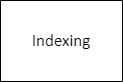
A step is a task, a semantic unit of processing such as “indexing,” which is when candidate record pairs for further processing are selected out of the space of all possible pairs. (This is closely related to blocking, in ways that will become clear later in this document.) A step is abstract, not tied to a specific algorithm to achieve the task; therefore, a step can be performed by many different implementations.
We draw a step as a box and label it with its name:
Default Implementations
A step with a check mark on its top right corner has a default implementation. Therefore, the user doesn’t have to specify anything. If the user wants to, they can override the default implementation. We draw these steps in gray.
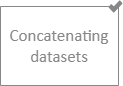
This is useful because some steps in the record linkage process are quite straightforward and unlikely to be sites of innovation. Default implementations for these allow EasyLink users to focus on the more interesting steps without taking away any flexibility— if there is some unexpected need to use new implementations for these less-interesting steps, the user can do that.
Slots
A slot is a semantic type of data that a step either receives or produces.
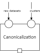
For example, consider “canonicalization,” which is a step in record linkage that produces a “canonical” record for each entity (e.g., each person). An implementation of this step might contain a specific algorithm for choosing which of the first names a person reported in different datasets to use in that person’s canonical record. This step needs to receive two types of input: clusters of record IDs that correspond to the same entity, and the full datasets (from before linking) to pull possible values from. These two types of input are not interchangeable— any implementation of the step needs to know which is which. Therefore, they go in different labeled slots.
We draw input slots (slots for receiving data) as small circles on the border of a step. We draw output slots (slots for producing data) as small squares on the border of a step. A step may have multiple of either or both.
A data specification is a set of rules that data can be validated against.
Every slot is associated with a data specification
that any data passing through it must follow.
It isn’t enough to say that a particular dataset is “clusters of record IDs”—
it has to actually look how we would expect those to look.
This could include constraints like having a specific tabular schema,
uniqueness in certain fields, etc.
For example, “clusters of record IDs to canonicalize” might entail
having two columns, record_id and cluster_id,
and record_id must be unique.
The label on the arrow (e.g., “raw datasets” or “clusters”) indicates the data specification that the data must follow (this label is implicitly applied to any slots it is connected to). The actual description of the data specification is not included in the diagram; that will be listed in text below it.
Though we may expand this in the future, we currently think of data in terms of files or directories. Directories may be nested. Here are some random examples of how data specifications could look, to show the breadth of possible specifications:
“A single file in a tabular format with columns A, B, and C.”
“A directory containing three files, where each is in a tabular format and has three columns.”
“A directory containing any number of subdirectories. Each subdirectory must contain two files, where each is in a tabular format.”
Data specifications are enforced by EasyLink; a pipeline will fail if any data do not follow their specification.
Data Dependencies
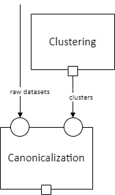
We connect an output slot to an input slot with an arrow, as shown below, when the output of one step becomes the input to another.
Note
There cannot be loops/cycles of data dependency (e.g., A -> B -> A), as then there would be no possible order to run the steps in – you couldn’t run A until you had B’s output, but couldn’t run B until you had A’s output!
Pipeline Schema
A basic pipeline schema is a set of steps interconnected by data dependencies that additionally has input data nodes (large circles) and output data nodes (large squares with bold text).

This is a graph in the computer science/mathematical sense. More specifically, it is a directed (arrows have a direction) acyclic (no arrow loops as discussed in the previous section) graph (DAG).
The text labels in input and output nodes, like the labels on dependency arrows, indicate data specifications the input/output data must follow (they implicitly label the slots they are connected to by dependency arrows.)
Data for the input nodes of the pipeline schema are provided directly by the user. An input node can have a check mark on it to indicate that it has a default:

Such an input can be omitted by the user, in which case the default value/dataset is used. This is useful, for example, when it would be common for the user not to have any data for that input: rather than having to manually make a data frame with zero rows and pass it in, they can simply omit it from their configuration.
However, a pipeline schema can contain more than just input, output, steps, and dependencies. It can have some additional tricks, which we call operators. These allow a pipeline schema to be more flexible and contain patterns that the user (or EasyLink itself) can customize to change the shape of the graph before selecting implementations. These operators are the subject of the next section.
Operators
Todo
Consider replacing the examples in this section with extracts from the record linkage pipeline schema, as in the previous section.
Cloneable sections
A section of a pipeline schema can be marked as cloneable. This means that some number of copies of that section will be created, with no data dependencies between the copies (so they look like “parallel tracks”). The EasyLink user chooses how many parallel copies of the section they want, and they can specify different implementations for each copy.
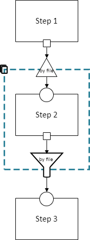
A cloneable section is marked by a dashed blue rectangle with a “clone” icon at the top left:
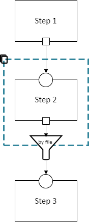
Every data dependency that passes from inside a cloneable section to outside it must have a specified method for aggregating the multiple outputs (one from each copy) back into a single output for the downstream (dependent) steps. This is indicated by the funnel in the diagram, which is labeled with the aggregation method.
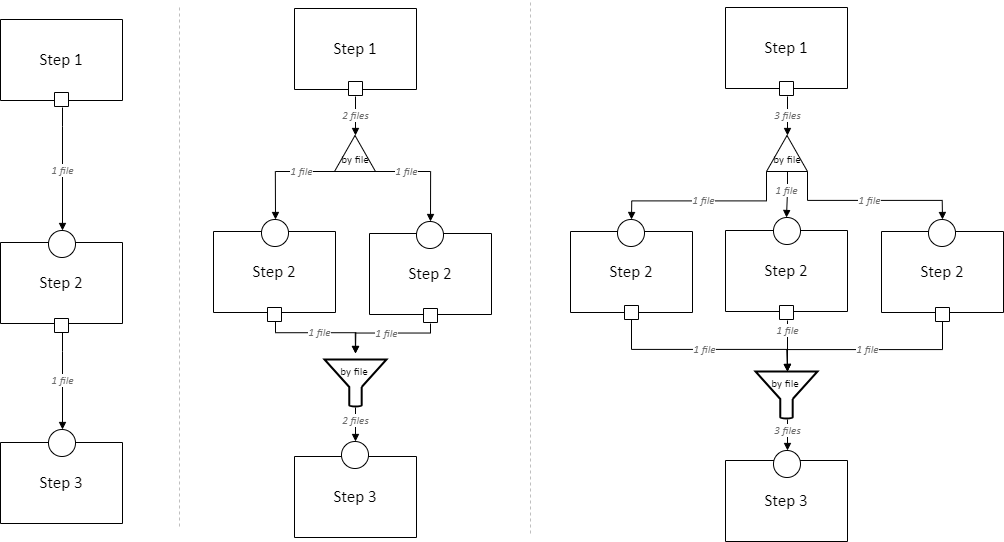
This diagram indicates that any of the following pipelines are permitted:
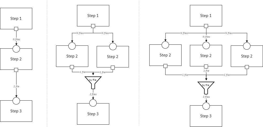
And on and on, with any number of copies of Step 2. The “by file” aggregator here takes multiple outputs (which may each be directories containing multiple files) and combines them into a single flat directory of files (the labels on the arrows in gray show the number of files in each directory in our example, to illustrate this). Other combination methods are permitted; this is just an example.
Loop-able sections
A loop-able section is a part of a diagram that can repeat as many times as the user configures, with some data dependency between iterations.
A loop-able section is denoted by a red dashed box:
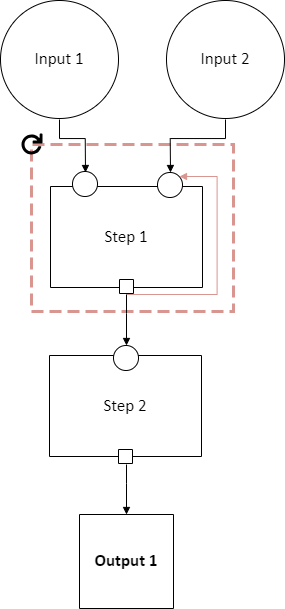
This diagram indicates that Step 1 may repeat an arbitrary number of times. The red arrow from the output slot of Step 1 to its “Input 2” input slot indicates that the output of Step 1 replaces “Input 2” in the next iteration. The black arrow from the output slot to Step 2 indicates that the output of the last iteration of Step 1 goes there.
In diagram form, that means the loop can expand in any of these ways:
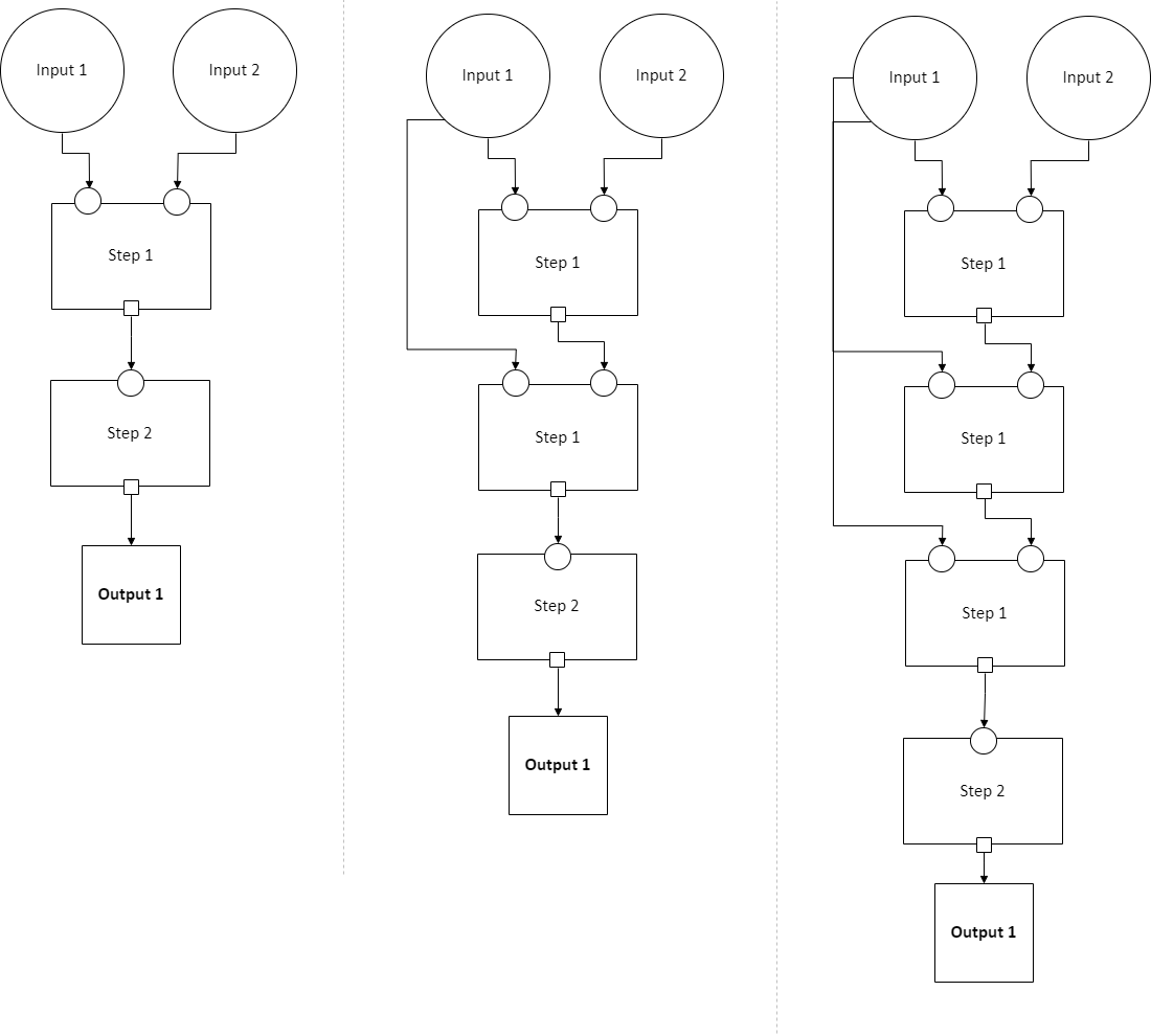
And on and on, with any number of copies of Step 1, chained in sequence.
The EasyLink user (the pipeline creator) chooses how many iterations of a loop-able section there are and may select different implementations for each iteration.
Splitters
There may optionally also be a method to split a single data dependency as it enters any kind of section. In the example from the cloneable section above, there was no splitter, so a copy of Step 1’s entire output would be given to each implementation of Step 2.
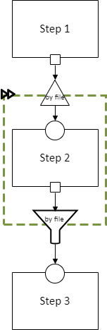
Splitters are represented by triangles on the border of the section, shown here with a cloneable section:
Which is expanded like so:
The “by file” splitter takes an input directory of N files and transforms it into N separate paths to each file. Other split methods are permitted; this is just an example.
Note that when there is a splitter, the number of splits created from the input data dependency must be equal to the number of copies of the section. For example, in the rightmost example above, there must be 3 files in the directory, in order to be split 3 ways for the 3 copies of Step 2.
Because this requires the number of copies/iterations of the section to be specified up front, a splitter can only be used if the number of splits is known before executing any implementations (i.e. the pipeline’s original input data are being split, or the data dependency that is being split has a data specification that guarantees the number of splits that will be made).
Auto-parallel sections
Auto-parallel sections are nearly identical to cloneable sections; they also indicate that a section can be copied multiple times without data dependencies between the copies.
The key differences are that auto-parallel sections are automatically expanded by EasyLink itself (the user doesn’t configure anything) and the same implementations are used in each copy.
Auto-parallel sections are intended for embarrassingly parallel computations, where the result does not meaningfully change regardless of the number of splits. Exactly one input data dependency must have a splitter, and EasyLink will decide at runtime how to optimize performance by splitting the data into chunks (using heuristics that have yet to be designed, involving file size, etc.). The number of parallel copies of the section will match the number of data chunks, and each parallel copy will use the same implementations.
Auto-parallel sections are denoted by green boxes with fast-forward icons:
Choice sections
A choice section allows the EasyLink user to choose one of several options, where each option is a section of the diagram. Everything in the other options, and any arrows from/to it, “disappears” for the purposes of the user’s pipeline. In other words, it is as if the pipeline schema only included the diagram section of the chosen option, and none of the other options.
A choice section is represented by an outer yellow dashed box, and a separate inner yellow dashed box within it for each option:
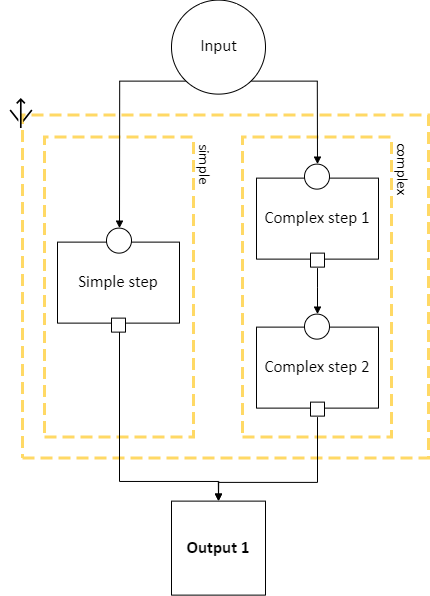
Here, the labels “simple” and “complex” on the inner dashed boxes are the names of the options.
With the above pipeline schema, the user could either choose “simple” or “complex”:
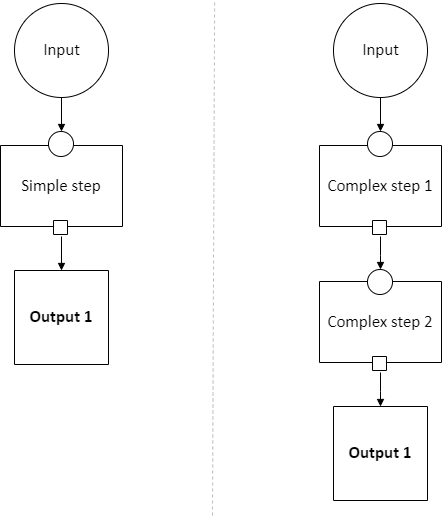
Step hierarchy
Pipeline schemas are self-similar: they have input and output nodes, just like each step within them has input and output slots.
Each step can also contain a graph of steps. If it does, this means that the user can either assign that step a single implementation, or the user can “zoom in,” resolve operators in the sub-graph, and then assign an implementation to each sub-step. Each input slot on a step becomes an input node, and each output slot on a step becomes an output node, in the graph of its sub-steps.
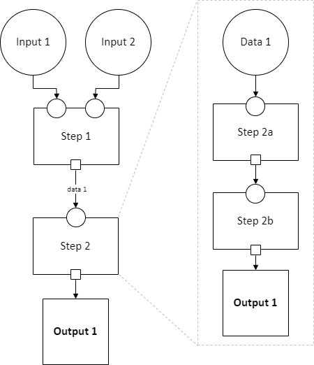
Note
There are no other operators in this example for simplicity, but remember that all operators are permitted to appear in sub-step diagrams!
The hierarchy can be nested arbitrarily deep: for example, Step 2a on the right might also have sub-steps. Because this can get so complicated, we don’t show all the hierarchical levels in one diagram as we’ve done above with the dotted line “insert.” Instead, we make a separate diagram with the title “Step 2” that represents the step graph contained within Step 2. In this diagram, we show a little “mini-map” of the levels of hierarchy above, highlighting in red the step that we are diagramming the inside of. Think of this like a “You are Here!” label.
At the top level of the step hierarchy, the pipeline schema splits the entity resolution task into very coarse steps, but lower levels in the hierarchy subdivide those and so on. The more detail in the pipeline schema that is used, the more interoperability and standardization the user gets.
Pipelines
The pipeline schema defines the universe of pipelines that can be constructed using EasyLink. To construct a pipeline, the user specifies how to resolve all the operators in the pipeline schema (except for auto-parallel sections, since these are resolved by EasyLink automatically). The result is a graph consisting only of inputs and outputs, steps, data dependencies, and auto-parallel sections; all loop-able sections have been unrolled, cloneable sections have been expanded, etc. In such a graph, each step requires an implementation, and the user specifies these (unless there is a default implementation, in which case that is used if the user doesn’t override it). Once this is complete, the result is the pipeline graph, which is ready to be executed.

Combined implementations
There is one additional trick that can be present in the pipeline graph, which allows both users and implementation authors more flexibility, in accordance with EasyLink’s “bend, don’t break” design principle.
Typically, an implementation implements a single step, at some level of detail in the pipeline schema. However, in some cases this may not be flexible enough. To accommodate this, we allow implementations to implement any subgraph in the pipeline – any set of nodes in the pipeline graph – provided that subgraph can be merged into a single node without introducing dependency cycles. This allows an implementation to perform multiple steps at once, sharing information between tasks. This harms interoperability, since it is no longer possible to substitute the individual steps, so combined implementations are discouraged except when absolutely necessary.
Let’s look a little more concretely at how this works. Instead of each step (after resolving operators) being assigned a different implementation, some steps are configured to be implemented with a combined implementation. Data dependencies between these steps are removed, and then the step nodes are merged.

EasyLink pipeline schema
Datasets
Interpretation: A set of named datasets. Each dataset contains observations recorded about (some) entities in the population of interest for analysis.
Specification: A directory of files, where each file is in a tabular format. Each file’s name identifies the name of that input dataset. Each file may have any number of columns, but one of them must be called “Record ID”. Values in the “Record ID” columns of each file must be unique integers.
Example:
A directory containing two files, input_file.parquet and reference_file.parquet.
input_file.parquet has contents:
Record ID |
First |
Last |
Address |
|---|---|---|---|
1 |
Vicki |
Simmons |
123 Main St. Apt C, Anytown WA 99999 |
2 |
Gerald |
Allen |
456 Other Drive, Anytown WA, 99999 |
reference_file.parquet has contents:
Record ID |
First |
Last |
Address |
|---|---|---|---|
1 |
Victoria |
Simmons |
123 Main St. Apt C, Anytown WA 99999 |
2 |
Gerry |
Allen |
456 Other Drive, Anytown WA, 99999 |
Known clusters
Interpretation: If any clusters are already known, they can be provided here (format described in “Clusters” sub-section). This is typically empty, which is the default, representing that there is no prior knowledge of clusters (all records are unresolved).
Clusters
Interpretation: A (partial) clustering of the input records, which indicates that records assigned the same cluster ID are observations of the same entity and records with different cluster IDs are observations of different entities. Records without a cluster ID are unresolved (they may or may not be part of one of the existing clusters).
Clusters are similar to pairwise links (described in more detail below) but inherently enforce the logical consistency of transitivity – if A and B are in the same cluster, and B and C are in the same cluster, then A and C are in the same cluster by definition.
Specification: A file in a tabular format with three columns: “Input Record Dataset”, “Input Record ID”, and “Cluster ID”. Combinations of values in the “Input Record Dataset” and “Input Record ID” columns must be unique. “Cluster ID” may take any value.
Note
In the future, we should add to this specification that each “Input Record ID” is a Record ID value found in the input dataset indicated by the “Input Record Dataset” column. EasyLink currently doesn’t support this.
Example:
Input Record Dataset |
Input Record ID |
Cluster ID |
|---|---|---|
input_file |
1 |
1 |
input_file |
2 |
2 |
reference_file |
1 |
2 |
input_file |
4 |
3 |
input_file |
5 |
3 |
reference_file |
2 |
3 |
In this example, record ID 1 in dataset “input_file” has been put in its own cluster, meaning that it does not match any of the other records listed. input_file record 2 has been put in a cluster with reference_file record 1, indicating that they refer to the same person. input_file record 3 doesn’t appear in the table at all, meaning that its cluster is unknown. Lastly, input_file record 4 and input_file record 5 are considered duplicates (records, from the same data source, referring to the same entity) and are also a match to reference_file record 2.
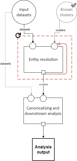
Entity resolution
Interpretation: Resolving (some) records to correspond to particular entities. A set of records corresponding to the same entity is called a “cluster.”
This step may take into account already-known clusters as it sees fit: anything from using them as a starting point for optimization to treating those clusters as set-in-stone and unchangeable.
Typically, this would only be be performed once, but the red dashed box in the diagram above indicates that it may be looped, with the clusters found in each iteration passed on to the next. This allows for one kind of cascading, an iterative approach to entity resolution used by the US Census Bureau (and possibly other organizations too) to deal with the computational challenge of linking billions of records. In cascading, multiple passes are made to find clusters, starting with faster techniques (such as exact matching) that can solve some “easy” cases and make the problem smaller. As the focus narrows to only the records that are hardest to cluster, making the size of the problem smaller, more sophisticated and computationally expensive techniques can be used.
Todo
Give cascading its own documentation page?
The sort of cascading represented by the looping section in this diagram is the kind in which a clustering (guaranteed to satisfy transitivity) is confirmed before moving to the next iteration. There is another kind of cascading, in which pairwise links are confirmed but transitivity is not enforced. That kind of cascading is represented by the looping section in the sub-steps of clustering, which nests within this entity resolution step.
This step has sub-steps, which may be expanded for more detail.
Examples:
The US Census Bureau’s Person Identification and Validation System (PVS) modules are considered entity resolution passes, since full clusters – called “protected identification keys” (PIKs) in that system – are resolved in between modules (not only pairwise links!). As described below, each module only considers records not already clustered.
In FIRLA and similar incremental methods, the already-found clusters would be used directly and updated with new decisions about not-yet-clustered records.
Canonicalizing and downstream analysis
Interpretation: Everything else you want to do, after determining which records belong to the same entity and which don’t. This definition is a little fuzzy. The downstream task is only included in the pipeline schema at all so that combined implementations can jointly do part of the entity resolution task with the downstream task, each informing the other. If this kind of joint model isn’t necessary, this step can simply output entire datasets to leave options open for later analysis.
Examples:
In PVS, the downstream task is not included in the pipeline, and this step would simply attach the PIKs (cluster IDs) to the input file (which is one of the two input datasets) and then output the entire file
Fitting a linear regression and outputting association statistics
Estimating population size and outputting a single number
Analysis output
Interpretation: The result of the analysis, whatever that may be. Could be a single statistic, a set of statistics, a whole dataset, or multiple datasets.
Specification: None. May take any form.
Entity resolution sub-steps
The direct sub-steps of entity resolution mostly have to do with cascading and incorporating already-known clusters, both of which are rare situations. All of the steps except for clustering have default implementations and are not relevant in the common situation of starting from scratch (no known clusters) and clustering in one pass (no cascading). For this reason, clustering is described first below.

Clustering
Interpretation: Assigning cluster IDs to (some) records to indicate which correspond to the same entity. May use information about “old” clusters as a starting point.
This step has sub-steps, which may be expanded for more detail by pairwise methods. Methods that are not pairwise should implement this step directly.
Examples:
The core part of a PVS module
dblink (would ignore “old” clusters, since there is no way for it to update)
In Splink, this step would correspond to estimating parameters, making pairwise predictions, and then clustering entities with connected components or similar
Dataset
Interpretation: A single dataset, see “datasets”.
Specification: A single file, which follows exactly the specification of each file in the directory of “datasets”.
Determining exclusions
Interpretation: Identify records that can be excluded from the input datasets for the purposes of this pass to save computational time. Usually these will be records that have already been clustered sufficiently well (whatever that means as defined by the implementation of this step) that we don’t need to look at them anymore.
Default implementation: Throws an error if there are any known clusters. Otherwise, returns an empty list (no records to eliminate).
Example: As mentioned above, our main example of entity resolution passes is PVS modules such as NameSearch, DOBSearch, etc. In those modules, the implementation of this step would be to eliminate all input-file records that are already linked to at least one reference-file record.
IDs to remove
Interpretation: Input record IDs slated to be dropped from a given dataset for the purposes of this pass.
Specification: A single file in tabular format, with exactly one column called “Input Record ID”. Every value in the column should be unique.
Note
In the future, we should add to this specification that each “Input Record ID” is a Record ID value found in the input dataset corresponding to this IDs to remove – that is, the one that was passed to “determining exclusions.” EasyLink currently doesn’t support this.
Example:
Input Record ID |
|---|
2 |
4 |
Removing records
Interpretation: Actually removing records slated to be dropped.
Default implementation: Pandas code dropping records with matching record IDs. Note that if the default implementation is used, input and output data specifications do not need to be checked.
Dataset (in directory)
Interpretation: A directory containing a single named dataset. See “datasets”. This is only different from “dataset” so that an implementation can output a dataset with a name (because, for file outputs, the name is fixed).
Specification: A directory containing a single file, which follows exactly the specification of each file in the directory of “datasets”. The name of the file is the name of the dataset.
New clusters
Interpretation: Clusters generated by this pass. May include some or all of the same records as the “old” clusters.
Specification: See specification for “Clusters.”
Updating clusters
Interpretation: Updating/reconciling previously-found clusters with newly-found clusters.
Default implementation: Throws an error if there are any known clusters. Otherwise, returns the new clusters unchanged.
Examples:
In PVS, simply appending PIKs found in this module to those found in previous modules. Because of the “determining exclusions” strategy used in PVS, these are guaranteed to not include any of the same input file records.
A simple approach would be to make each set of clusters into a graph of records, merge the graphs, and take the connected components as the updated clusters.
Clustering sub-steps
As mentioned above, the sub-steps of clustering are designed for pairwise methods – models of entity resolution that only consider pairs of records at a time. Breaking down the entity resolution task into a binary classification problem about whether or not each pair of two records belong to the same entity simplifies it enormously, and traditional methods going back to Fellegi and Sunter (1969) take this approach.
Methods that are not pairwise will need to implement the “clustering” step as a whole, as they are not composed of parts that align with these sub-steps.
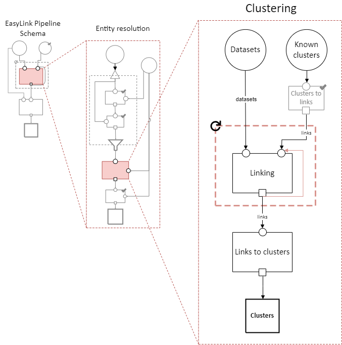
Clusters to links
Interpretation: Converting clusters (sets of records that are all mutually linked) to links (pairs of records that are linked).
Default implementation: Pandas code that generates all the unique (unordered) pairs of records within each Cluster ID group, and pairs them with probability 1.
Links
Interpretation: Pairs of records that are linked with some probability.
Links can be seen as another way to represent the same information as clusters, but links are not conducive to enforcing the structural constraint of transitivity: that if A links to B and B links to C, A must link to C. This lack of structural awareness is inherent to pairwise methods, and the loss of information this represents is a tradeoff with the benefits of the simplicity of the pairwise approach to entity resolution.
Assigning a probability to each pair is an efficient system for representing uncertainty, when the statistical dependence structure between the pairwise links is unknown. It is up to downstream steps to interpret/assume the dependence structure between pairwise probabilities. If a method doesn’t represent uncertainty, it can set all probabilities to 1 (or another constant).
Specification: A table with five columns: “Left Record Dataset”, “Left Record ID”, “Right Record Dataset”, “Right Record ID”, and “Probability”. It is not permitted for Left Record ID to equal Right Record ID and Left Dataset to equal Right Dataset in any given row. The combination of the four columns besides Probability should be unique (i.e. multiple rows with the same Left Record Dataset, Left Record ID, Right Record Dataset, and Right Record ID would not be permitted). The Left Record Dataset value should be alphabetically before (or equal to) the Right Record Dataset value in each row. In rows where Left Record Dataset and Right Record Dataset are equal, the Left Record ID value should be less than the Right Record ID value. (These two rules ensure each pair is truly unique, and not a mirror image of another.) Each value in the Probability column must be between 0 and 1 (inclusive).
Note
In the future, we should add to this specification that every value in both Record ID columns should exist in the corresponding input datasets. EasyLink currently doesn’t support this.
Example:
Left Record Dataset |
Left Record ID |
Right Record Dataset |
Right Record ID |
Probability |
|---|---|---|---|---|
input_file |
2 |
reference_file |
3 |
0.9 |
input_file |
2 |
reference_file |
4 |
0.8 |
input_file |
3 |
reference_file |
6 |
0.4 |
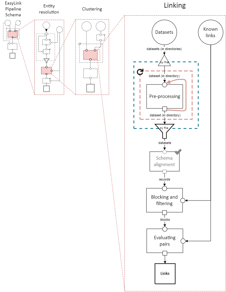
Linking
Interpretation: Finding pairs of records that should be considered links (correspond to the same entity).
Typically, this would only be be performed once, but the red dashed box in the diagram above indicates that it may be looped, with the links found in each iteration passed on to the next. This allows for the other kind of cascading, an iterative approach described above.
The sort of cascading represented by the looping section in this diagram is the kind in which links are confirmed before moving to the next iteration. There is another kind of cascading, in which clusters are confirmed and transitivity is enforced. That kind of cascading is represented by the looping section in the top-level pipeline schema.
Examples:
A single PVS pass within a module, such as the first pass of GeoSearch, which as of 2014 used blocking on the Master Address File (MAF) ID.
In Splink, this step would correspond to estimating parameters and making pairwise predictions (possibly with a threshold)
Links to clusters
Interpretation: Converting links (pairs of records that are linked) to clusters (sets of records that are all mutually linked).
This implies resolving issues with transitivity: if A links to B and B links to C, A must link to C. Resolving these issues requires making after-the-fact corrections to some of the links found, taking advantage of the context provided by other links. Making these corrections outside the linkage model is not ideal, but this is the price paid in return for the simplicity of the pairwise approach.
Clusters are also much more conducive to representing other structural constraints the analyst may have, such as a one-to-one link between two files. We expect that these constraints will typically be enforced during this step.
Examples:
The simplest algorithm is finding the components (also called “connected components”) of the graph created by giving every record a node and every pair (with probability above a threshold) an edge. This is implemented in Splink.
In PVS, the algorithm incorporates the restriction that multiple records from the reference file should never be in the same cluster. Therefore, the links are filtered before going into connected components: only the link with the highest probability for each input file record is kept, and if there are ties for the highest probability, no links involving that input file record are kept. This is described here as a “post-search program.”
In other Census Bureau processes such as the linkage of the Post Enumeration Survey (PES) to the Census, there is a 1-to-1 restriction: there can only be one record from each file in a cluster. This is achieved by finding the matching such that the sum of the (logit) probabilities of the accepted matches is maximized, as described in Jaro (1989).
Note
None of the methods in this list are able to propagate the uncertainty represented by the pairwise probabilities through this step, e.g. by sampling clusters somehow. Further research is needed in this area.
Linking sub-steps
Used in this diagram and defined above:
Pre-processing
Interpretation: Performing data cleaning steps on a given dataset, such as standardizing abbreviations, replacing “bad” data with missing values, etc.
Note that this step is for operations that are applied independently to one dataset at a time. For cross-dataset operations, see Schema alignment.
The loop-able section around this step allows it to be looped an arbitrary number of times, so that multiple cleaning steps can be performed on the same dataset.
Examples:
An address standardizer
Adding nicknames/alternate names
Replacing fake names such as “DID NOT RESPOND” with NA/null
Renaming columns or dropping empty columns from a dataset
Schema alignment
Interpretation: Aligning data formats across all datasets to facilitate linkage.
Typically, in administrative data practice, the analyst will manually determine what cleaning steps need to be applied to all the datasets to make them consistent with each other. If those cleaning steps are all performed in pre-processing, then the datasets would already have the same columns (and consistent value formats within those columns) before this step. In that situation, there is nothing difficult left to do here and the default implementation described below is all that is needed.
In the computer science literature, however, there are emerging methods for doing this alignment automatically. If desired, datasets could be passed into this step still inconsistent with one another, and a model could run in this step to automatically complete the alignment by figuring out which columns correspond to each other and how to standardize values.
Default implementation: Pandas code that simply concatenates the datasets, matching columns by name, and appending information about the dataset each record came from. In code:
import pandas as pd

def schema_alignment(datasets: dict[str, pd.DataFrame]) -> pd.DataFrame:
   return pd.concat([
      df.assign(
         dataset=dataset,
      ).rename(columns={"Record ID": "Input Record ID"})
      for dataset, df
      in datasets.items()
   ], ignore_index=True, sort=False)
Examples:
The Unicorn model contains automatic schema alignment.
Records
Interpretation: The records to link (from all datasets) in one big table.
Specification: A file in a tabular format. The file may have any number of columns, but they must include “Input Record Dataset” and “Input Record ID” and the combination of those two columns must have unique values.
Note
In the future, we should add to this specification that every value in the Input Record ID column should exist in the corresponding input dataset. EasyLink currently doesn’t support this.
Example:
Input Record Dataset |
Input Record ID |
First |
Last |
Address |
|---|---|---|---|---|
input_file |
1 |
Vicki |
Simmons |
123 Main St. Apt C, Anytown WA 99999 |
input_file |
2 |
Gerald |
Allen |
456 Other Drive, Anytown WA, 99999 |
reference_file |
1 |
Victoria |
Simmons |
123 Main St., Anytown WA 99999 |
reference_file |
2 |
Gerry |
Allen |
N/A |
Blocking and filtering
Interpretation: Breaking the linkage problem up into pieces that can be tackled separately, and selecting which pairs of records to consider in each piece, in order to reduce the size of the task and therefore the computation required.
Traditional blocking, where a blocking “key” is assigned to each record, implements this step by splitting the records into blocks (disjoint subsets) by their blocking key and enumerating all possible pairs within each block.
More advanced techniques may instead create just one block (with all records), and select only some pairs within that block rather than every possible pair.
Techniques focused on or configured for linkage between datasets can avoid enumerating pairs of records within the same dataset.
This step corresponds to “indexing” in Christen (2012).
Examples:
In Splink, using a single blocking rule would be traditional blocking as described above: a separate block for each value of date of birth, for instance. Multiple blocking rules in Splink are OR’d together, creating overlapping blocks. In EasyLink, this could be represented as putting all records in a single block but only enumerating the pairs matching at least one of the blocking rule conditions.
Blocks
Interpretation: Separate pieces of the linkage task that can be tackled separately, along with the pairs of records to consider in each.
Specification: A directory containing any number of subdirectories. Each subdirectory must contain two files, each in tabular format: records and pairs.
Each records file must follow the specification for Records.
Each pairs file must contain four columns: “Left Record Dataset”, “Left Record ID”, “Right Record Dataset”, and “Right Record ID”. Every combination of values in Record Dataset and Record ID columns (left or right) should exist in the records file for the same block. It is not permitted for Left Record ID to equal Right Record ID and Left Dataset to equal Right Dataset in any given row. Rows should be unique (i.e. multiple rows with the same Left Record Dataset, Left Record ID, Right Record Dataset, and Right Record ID would not be permitted). The Left Record Dataset value should be alphabetically before (or equal to) the Right Record Dataset value in each row. In rows where Left Record Dataset and Right Record Dataset are equal, the Left Record ID value should be less than the Right Record ID value. (These two rules ensure each pair is truly unique, and not a mirror image of another.)
Note
The specification for each pairs file is identical to the specification for Links except that there is no probability column.
Example:
The overall directory tree structure might look like:
blocks
├── block_0
│   ├── pairs.parquet
│   └── records.parquet
└── block_1
   ├── pairs.parquet
   └── records.parquet
A records file might look like:
Input Record Dataset |
Input Record ID |
First |
Last |
Address |
|---|---|---|---|---|
input_file |
1 |
Vicki |
Simmons |
123 Main St. Apt C, Anytown WA 99999 |
input_file |
2 |
Gerald |
Allen |
456 Other Drive, Anytown WA, 99999 |
reference_file |
1 |
Victoria |
Simmons |
123 Main St., Anytown WA 99999 |
reference_file |
2 |
Gerry |
Allen |
N/A |
A pairs file might look like:
Left Record Dataset |
Left Record ID |
Right Record Dataset |
Right Record ID |
|---|---|---|---|
input_file |
2 |
reference_file |
2 |
input_file |
2 |
reference_file |
4 |
input_file |
3 |
reference_file |
6 |
Evaluating pairs
Interpretation: Determining a link probability for each pair of records based on those records’ values. This transforms pairs (which are simply two record IDs) into the format of Links, which include this probability.
Examples:
In Splink, training the model, calculating the comparison levels, and predicting the match probability
fastLink’s entry method, assuming the set of pairs is exhaustive (fastLink currently has no way to limit pairs)